When to Rebalance

When following an asset allocation scheme there are two issues to consider: how frequently to check the current asset allocation against the recommended asset allocation, and then whether to rebalance. For whether to rebalance, we use the idea of a rebalancing band. We rebalance back to the recommended asset allocation only if the distance of any of the asset classes of the current asset allocation from the recommended asset allocation is equal to or greater than the rebalancing band half width.

The initial scenario used is a 25 year old male just beginning to save for retirement at age 65, making withdrawals until death, and performing asset allocation using Stochastic Dynamic Programming (SDP) all as described more fully at the end of this posting. We record how rebalancing frequency and rebalancing band half width effect portfolio failure. Portfolio failure is defined as the portion of the individual's remaining lifetime for which they are insolvent.

We simulate a number of different rebalancing check frequencies, and a number of different rebalancing band half widths, and graph portfolio failure as a function of these two variables. We simulate 100,000 returns sequences for each data point.

The portfolio failure percentage when drawing returns at random form the historical record are shown below, with lines drawn to connect data points with the same rebalancing check frequency.

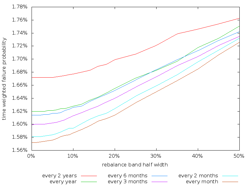
Nothing unexpected here. The more frequently rebalancing is checked and the narrower the rebalancing band half width the better the performance. The optimal performance is to check monthly with a rebalancing band half width of 0%.

But wait...

That was when selecting individual monthly returns at random.

Things get a lot more interesting when we evaluate rebalancing using returns sequences composed of 20 year blocks of data drawn from the historical record. This is shown below.

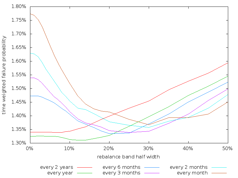
With no rebalancing band (half width 0%) monthly rebalancing now performs worst, and annual rebalancing now performs best. The shorter time period rebalancing lines also now have a dip located somewhere around 20-30% where they perform best. What is going on?

One possible explanation is momentum of some sort. Momentum has been well studied in individual stocks, but less so in aggregate asset classes. But the basic idea is clear. When the stock or bond market rises, it is likely to continue to rise. Rebalancing under such circumstances is likely to reduce the gains experienced. Similarly when the stock or bond market falls, it is likely to continue to fall. Rebalancing will only increase the losses. It is better to wait out the fluctuations of the market either by rebalancing less frequently or employing rebalancing bands.

Looking at the annual line, the best strategy appears to be to check annually and rebalance if an asset class differs from its target asset allocation by more than, say, 12-14%.

Also looking at the annual line, the failure rate for a 20% rebalancing band half width is 0.017% higher than the best value obtained. Estimating the life expectancy at age 25 as 56 years, this amounts to a mean expected 3 days of additional portfolio failure. Given rebalancing takes several hours to perform per year the portfolio loss associated with employing a 20% rebalancing band half width appears acceptable in this case.

Broadly similar results were obtained for a male age 65 with a $1m portfolio. Realance annually with a 12% rebalancing band half width if you want to be precise, or 16% if you are more lazy.

Aggregating these results gives the recommendation to rebalance annually with a 15% rebalancing band half width.

Attempting to generalize these results to asset allocation schemes other than Stochastic Dynamic Programming failed. In particular a similar experiment was performed for age minus 10 in bonds. Unlike the Stochastic Dynamic Programming algorithm, which generates the optimal asset allocation scheme assuming returns come from a known distribution that is independent over time (as used in testing here), age minus 10 in bonds is a sub-optimal asset allocation strategy. Thus increasing the rebalancing band half width actually produced a lower failure probability, presumably because it allowed the portfolio to stay more heavily weighted towards stocks for longer, and for the scenario under consideration this was a better asset allocation scheme.

Scenario. We consider a male initially saving $2,000 at age 25, growing by 7% real per year, until age 65 at which point they retire and withdrawal a fixed real $50,000 per year. Money is added/withdrawn at the then current asset allocation. Longevity is as specified by the U.S. Social Security Cohort Life Tables for a person of the given initial age in 2013. Stock and bond market data for 1872-2012 are as supplied by Shiller (Irrational Exuberance, 2005 updated) without any adjustments being made. To evaluate each asset allocation scheme we generate 100,000 returns sequences using bootstrapping by concatenating together blocks of length 1 month or 20 years of monthly returns data chosen at random from the period 1927-2012. Rebalancing is performed at the indicated interval. No transaction fees. All calculations are adjusted for inflation. Taxes are not considered.

Asset allocation scheme. Asset allocation is performed using Stochastic Dynamic Programming (SDP). Asset allocation schemes are for U.S. stocks and 10 year Treasuries. SDP asset allocation was generated by first performing mean-variance optimization; not that is should make a difference. The SDP optimization goal was to minimize the time weighted odds of portfolio failure, not the pure odds of portfolio failure alone. Thus a portfolio failure length of 10 years is considered twice as bad as a portfolio failure length of 5 years. No value is assigned to leaving an inheritance. For SDP we use the period 1927-2012 as input data to generate an asset allocation map in blocks of the number of month being tested. This use of the same period to generate and evaluate makes the absolute performance questionable, but allows us to eliminate the difference between the generation and evaluation returns as a possible source of noise in the results.

Platform: An internal command line version of AACalc.com was used to generate the SDP asset allocation maps and simulate the scenarios.