Variable Withdrawal Portfolios Should Be Stock Heavy

All but 1-2 studies of variable withdrawal strategies assume a fixed asset allocation. And most studies of lifetime varying asset allocation strategies assume a fixed withdrawal amount. In practice it is common to combine variable withdrawal and time varying asset allocation strategies. However to get a meaningful handle on such combined strategies we can't simply combine the results from studying them separately. This is because variable withdrawals and time varying asset allocation conflict.

Conflict occurs when the outlook is rosy, and you are likely to have sufficient assets to live out your life expectancy. The benefits of variable withdrawals can then be maximized by a stock heavy portfolio, since it offers the greatest returns. Asset allocation by itself though wants to turn those surplus assets into portfolio safety, and so in the absence of valuing any bequest, favors bonds. In fact, the safest portfolio from an asset allocation perspective lies at the tip of the "Markowitz bullet" and is roughly 10% stocks and 90% bonds.

The conflict between the two goals can be resolved using Stochastic Dynamic Programming (SDP) to determine the best withdrawals and asset allocations for retirement portfolios. The results are surprising.

Results

Asset allocation strategy / withdrawal strategy.

Fixed / amount: For the decumulation scenario described more fully at the end of this note, the best fixed asset allocation and fixed withdrawal amount expressed in terms of the initial portfolio withdrawal rate are 50/50 and 3.6%.

Fixed / SDP: Switching to variable withdrawals computed using SDP, the best asset allocation jumps to 80/20. The use of a dynamic withdrawal model allows the portfolio to become more stock heavy.

SDP / Fixed: Using SDP to compute the asset allocation, but going back to a fixed withdrawal amount results in the best withdrawal amount of $37,000, and the following asset allocation map:

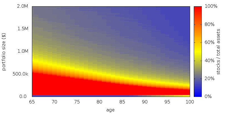
As can be seen, as the portfolio size increases, and the probability of success increases, the proportion of stocks drops, until it is somewhere around 10%. The artifact for portfolio sizes less than the withdrawal amount is a result of all choices being equally bad, and can be ignored.

SDP / SDP: Using SDP to compute the asset allocation and withdrawal schedule results in the following asset allocation map:

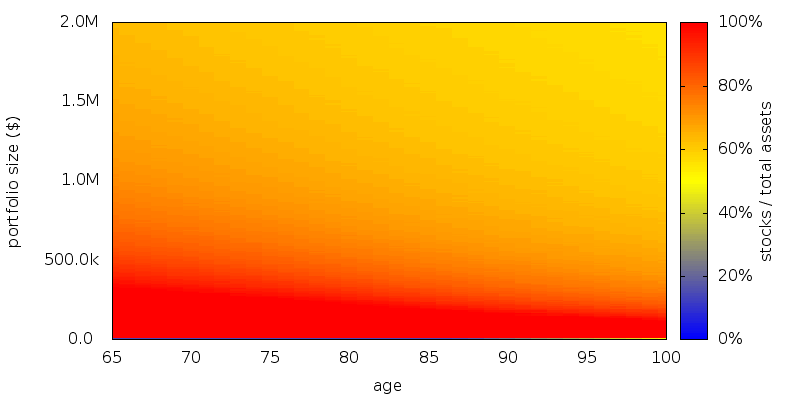
Sample portfolio paths are shown so that the region of the asset allocation maps that is utilized can be gauged.

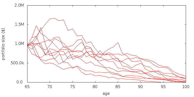
In the region of interest stocks range from 70 to 100%. This agrees with what we saw previously for a dynamic withdrawal model but fixed asset allocation.

These percentages of stocks are significantly higher than what is commonly recommended. For instance the S&P Target Date Retirement Income Index is 32% stocks, and the pre-retirement target date indexes range from 52-90% stocks (July 31, 2012 data). Which is itself considered high compared to the rule of thumb age in bonds, which posits 35% stocks at age 65, and decreasing from there.

Provided the aversion to insolvency is low enough, more benefit is obtained by consuming surplus assets than investing them in bonds for portfolio safety.

Conclusion

By combining variable withdrawals with asset allocation we get appear to get a significantly higher stock allocation than for asset allocation alone. Variable withdrawals act as a alternative to bonds by providing a financial release valve should stock returns be more or less than expected. Social Security or other defined benefits also act as an alternative to bonds by providing stability. With two sources of stability it is little wonder the investment portfolio itself can be allowed to be quite volatile.

Scenario

Scenario. A retired male/female couple, both age 65 with a $1,000,000 portfolio. $20,000 of guaranteed Social Security income is assumed. Longevity is as specified by the U.S. Social Security Cohort Life Tables for a person of the given initial age in 2013. No value is placed on any inheritance that is left. No additions to the portfolio are permitted, and withdrawals are made using the current asset allocation. Taxes were ignored. No transaction costs were assumed for rebalancing, sales, or purchases. All amounts are adjusted for inflation. No time discounting of the future is performed.

Asset allocation schemes: Rebalancing is performed annually. Returns data for 1927-2012 were used by SDP to generate the schemes. A zero consumption level of $0 was used, with 0% phase out with increasing income. We optimize a power utility function with a coefficient of relative risk aversion of 3.

Withdrawal schemes: Withdrawal are performed annually at the start of the year.

Asset classes and returns: U.S. stocks and 10 year Treasuries as supplied by Shiller (Irrational Exuberance, 2005 updated) but adjusted so the real return on stocks is 3.1% and bonds 0.1% before expenses. Management expenses are 0.1%.

Evaluation: For each retirement number value 100,000 returns sequences were generated by selecting returns at random from the period 1927-2012. In evaluating each sequence we compute the full range of longevity possibilities. For the fixed and amount schemes we selected the best results as the results with the highest certainty equivalence rate.

Platform: An internal command line version of AACalc.com was used to generate and evaluate the strategies.

Validation

In Spending flexibility and safe withdrawal rates, Finke et al. find the best allocation at 40/60 and 5% for a similar scenario. The difference can be explained by differences in death rates and market returns. Temporarily switching from the Social Security Administration cohort life tables to period life tables, to unadjusted historical returns, and no management expenses, all as used by Finke et al. produces a best allocation at 50/50 and 4.6%, or to be more precise at 45/55 and 4.5%, which agrees to the resolution of Finke et al., especially when allowing for small differences between the data sources.