Variable Withdrawals

There are many rules of thumb for variable withdrawal strategies which involve consuming more when times are good, and less when the future appears less rosy.

Rather than a rule of thumb it is also possible to compute an optimal variable withdrawal strategy if it is assumed annual returns are from a known distribution that is independent over time by using the Stochastic Dynamic Programming (SDP) algorithm. The requirement that returns be independent over time means SDP ignores volatility predictability, momentum, and reversion to the mean.

To compute the variable withdrawal strategy using SDP it is only necessary to treat the withdrawal amount as a dimension to be optimized over analogous to an asset allocation dimension. That is working backwards by age, for each portfolio size, we consider every asset allocation and withdrawal amount and pick the best one.

A typical withdrawal map is shown below.

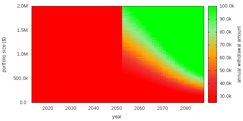
The year is displayed on the horizontal axis. Portfolio size is displayed on the vertical axis. And the recommended withdrawal amount is displayed color coded on the graph, as shown by the scale on the right. The left hand side of the graph shows the lack of withdrawals prior to retirement and can be ignored.

As can be seen the less rosy the outlook the smaller the withdrawal amount, and the more positive the outlook the bigger the withdrawal amount.

Performance

A variable withdrawal strategy reduces the odds of portfolio failure, but there is no free lunch. It achieves this reduction by reducing the well being derived from early period consumption if the future isn't looking so rosy. The question then becomes does the reduction in earlier period consumption more than offset by the increase in later period consumption.

Well being can be measured using a utility function, and we can use the inverse of this utility function to map the overall well being experienced back to a dollar value in order to make comparisons of well being more intuitive. When measuring well being experienced using a given asset allocation and withdraw map we perform a bootstrap simulation that does include volatility predictability, momentum, and reversion to the mean. For the data reported here, well being covers the accumulation as well as the decumulation phase, treating the accumulation phase as receiving welfare equivalent to the annual retirement withdrawal amount.

For concreteness we consider a male aged 25 who has just started saving for retirement as detailed more fully at the end of this article. Under this scenario with a fixed $50k annual withdrawal, the equivalent welfare amount annual withdrawal amount is $42,100. That is the individual is indifferent between the expected scenario outcome and receiving a guaranteed $42,100 per year until they die. Enabling variable withdrawals from $50k to infinity, the equivalent welfare amount is $43,600. That is by allowing consuming more when times are good things improve slightly. Enabling variable withdrawals from $25k to infinity, the equivalent welfare amount is $49,800. Consuming less when times are bad results in a significant improvement in overall welfare. Somewhat obviously, variable withdrawals reduce the odds of portfolio failure, here from 9.9% for fixed to 2.4% for $25k to infinity, but the improvement in welfare is less than that.

In the scenario just considered an extra dollar when you are broke was considered 100 times more valuable than an extra dollar when you were withdrawing the annual withdrawal amount of $50k. If an extra dollar is only 10 times as valuable a fixed $50k withdrawal amount gives an equivalent welfare amount of $47,800; a variable $50k to infinity gives $52,700; and $25k to infinity gives $54,600. This is quite different than the previous case. This time most of the improvement comes from enabling variable withdrawals on the high side, not the low side. In the first case we were saying running out of money is very bad, do everything possible to prevent it. This meant allowing variable withdrawals on the low side significantly increased utility. In the second case running out of money didn't matter so much, so it was possible to consume more on the high side without fear that might impact the future.

Stock heavy

An interesting observation regarding the variable withdrawals we have considered is their asset allocations tend to be very stock heavy. If normally bonds play an important role in stabilizing a portfolio, when variable withdraws are allowed they override this role to an extent; favoring the potential for increased consumption that comes with stocks over portfolio stability. This is especially true if poverty is only valued weakly.

Conclusion

In summary, variable withdraw strategies can reduce the odds of portfolio failure substantially, and improve welfare by a significant but lesser amount (remember our equivalent welfare values are lifetime amounts not retirement only amounts). This welfare improvement may come from reducing consumption when times are tough, or increasing consumption when times are good, possibly depending on the scenario and the sharpness of the utility function used.

Scenario

A 25 year old male initially with $0, saving $3,000 per year, and growing the savings rate by 7% real per year, until age 65 at which point they retire and withdrawal a fixed real $50,000 per year. Longevity is as specified by the U.S. Social Security Cohort Life Tables for a person of the given initial age in 2013. No value is placed on any inheritance that is left. Additions and withdrawals are made using the current asset allocation. Taxes were ignored. No transaction costs were assumed for rebalancing, sales, or purchases. All calculations are adjusted for inflation.

Asset allocation scheme. Rebalancing is performed annually. SDP is used to produce the asset allocation scheme. The optimization function was to maximize a power utility function on consumption. A zero consumption level of $10,000 was used, with zero phase out with increasing income. The annual withdrawal amount has a utility 100 or 10 times the zero consumption level. Returns data for 1872-1926 were used to generate the asset allocation map.

Asset classes and returns: U.S. stocks and 10 year Treasuries as supplied by Shiller (Irrational Exuberance, 2005 updated) but adjusted so the real return on stocks is 5.0% and bonds 2.1% before expenses. Management expenses are 0.5%.

Evaluation: 100,000 returns sequences were generated using bootstrapping by concatenating together blocks of length 20 years chosen at random from the period 1927-2012.

Platform: AACalc.com was used to generate the SDP withdrawal maps and simulate the scenarios.