How Much Does Asset Allocation Matter?

Asset allocation matters, but achieving the optimal asset allocation probably matters less than you might think. If you are using variable withdrawals then provided you adopt and stick with a high stock allocation you should do reasonably well.

Scenario

Consider a 65 year old male with a stochastic life span, no bequest motive, and receiving $15k/year in Social Security. Their stated floor consumption level is $30k/year, and they would like to consume an additional $10k beyond that. Above this they derive little utility from additional consumption. We model this with a coefficient of relative risk aversion of 4 up to $30k, dropping down to 1 above $40k. Floor consumption is considered 10 times more important than surplus consumption.

Since we are only concerned with math not psychology here, we consider the individual to have an unlimited risk tolerance, and do not impose a cap on the maximum stock holdings. However, we do not allow leverage.

For stocks we use the annual U.S. large cap returns and for bonds the 10 year Treasury returns for 1927-2014. The equity risk premium is 4.6% geometric mean. This is comparable to equity risk premiums predicted in the future. The returns for stocks are expected to be lower in the future but so are bonds, leaving the equity risk premium relatively unchanged. We are interested in the equity risk premium because it is what determines how much to allocate to stocks and how much to allocate to bonds according to the solution to Merton's portfolio problem.

Suppose the individual had perfect knowledge of the distribution of annual returns, but not their sequencing. Then there exists an optimal asset allocation and consumption strategy as a function of age and portfolio size. Moreover, provided the returns are independent over time, it is possible to compute this strategy using stochastic dynamic programming.

The future is discounted at a rate of 1.5% per year. Management expenses are assumed to be 0.1% per year. The individual wishes to maximize expected lifetime utility.

Life is not a glide path

The optimal allocation to stocks as a function of age and portfolio size computed using stochastic dynamic programming is shown below. This graph is a heat map. The optimal allocation is determined by first determining the color of the graph for a specified age and portfolio size, and then determining the asset allocation corresponding to that color using the color scale on the right.

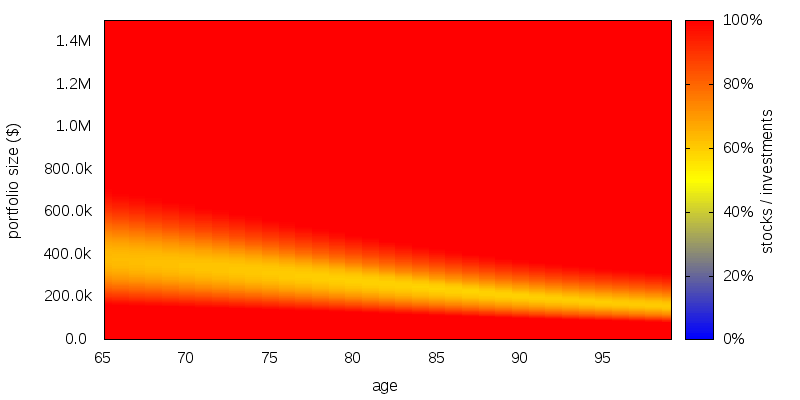
The bottom portion of the graph shows a 100% allocation to stocks. This is because the vast majority of the income is in the form of Social Security, which acts as a surrogate bond holding, and causes what otherwise would be a balanced allocation to tilt heavily towards stocks.

The top portion of the graph is again 100% stocks. This time because the low coefficient of relative risk aversion that prevails when you are wealthy allows more risk to be taken. In fact, ignoring Social Security, the allocation to stocks is inversely proportional to coefficient of relative risk aversion. This means the allocation to stocks should be 4 times what it is when consumption is below $30k.

In the middle is a more balanced asset allocation region.

The path the optimal asset allocation takes is not a smooth glide down one of these regions. This is because portfolio size is volatile. The figure below shows 10 sample portfolio paths for a starting portfolio size of $500k.

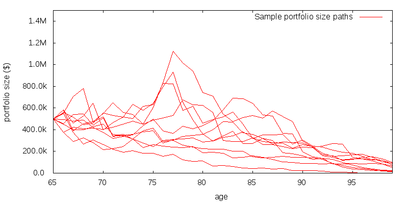
This portfolio size volatility creates significant volatility in the optimal asset allocation path. 10 sample asset allocation paths are shown below.

How much asset allocation matters

Following the optimal asset allocation is clearly a challenging task. What if we were off from the optimal stock allocation by a constant +20% every year, and bonds by -20%, while still consuming the recommended optimal consumption amount. How much would our average lifetime consumption utility be reduced as a result? To make the numbers involved tangible we make use of the concept of certainty equivalence, which is the constant consumption level having the same expected utility as a particular consumption sequence. From this we subtract Social Security to get the dollar amount of consumption that results from the portfolio investments. Then we compare the investment derived consumption to the investment derived consumption for the optimal asset allocation.

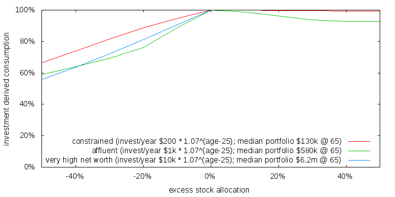
Computing the investment derived consumption for a range of initial portfolio sizes and excess stock allocations results in the following figure. Note that the lines for the constrained and affluent initial portfolio sizes to the right of the 0% excess stock allocation do not show because they are coincident with the top frame of the graph.

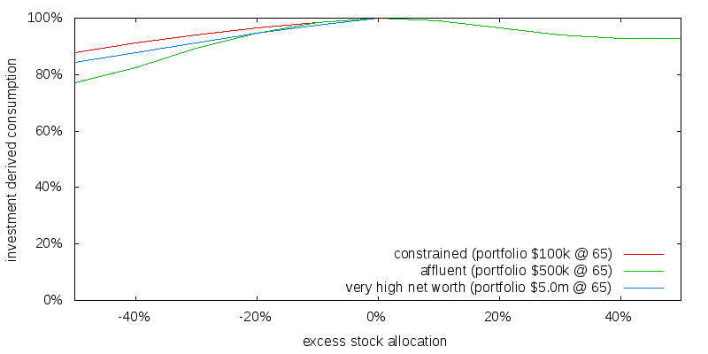
What this graph shows is the relatively low sensitivity of portfolio derived consumption to asset allocation. For the retiree a -20% mis-allocation to stocks, i.e. being 20% too bond heavy, will only result in a 4-5% reduction in investment derived consumption.

A +20% over allocation to stocks results in a 3% reduction for the affluent retiree, and 0% for the constrained and very high net worth retirees.

These results can be understood by looking at the sample asset allocation paths shown previously. The sample paths show stock allocations in the range 60-100%. Adding +20% to this range we will sometimes hit the 100% stocks cap, thus it is reasonable to expect reducing stocks to have a bigger impact than increasing stocks. The sample paths were for the affluent retiree. Referring to the stock asset allocation heat map we would expect the constrained and very high net worth retirees to have asset allocations much closer to 100% stocks. For this reason increasing the stock asset allocation barely effects performance.

What is the effect of the reduced utility of upside consumption?

We have been using a "floor and upside" utility function. What effect might this have? The figure below shows the asset allocation sensitivity using a constant relative risk aversion utility function with a coefficient of relative risk aversion of 4 everywhere.

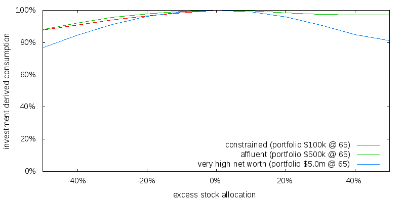
As might be expected the right hand side now shows the curve for the very high net worth individual. Apart from this though there aren't any major changes. A +/-20% change in asset allocation from optimal results in a 0-4% change in lifetime investment derived consumption.

Impact over a lifetime

So far we have only considered a retired individual. Getting things wrong over a lifetime we might expect to have a bigger effect.

We compute the optimal strategy for an individual age 25, no initial savings, and real investment savings contribution roughly doubling every decade until retirement. The approach we take isn't perfect. In particular retirement savings would probably best be described using a stochastic model rather than a fixed schedule. We chose the simple approach for expedience. But note a stochastic model would give future retirement savings a risky status potentially offsetting some of the need for high stock allocations. The impact of this expediency isn't known.

The figure below shows that a 20% over allocation to bonds results in a 11-24% impact on portfolio derived consumption. Meanwhile a 20% over allocation to stocks results in only a 0-4% reduction in portfolio derived consumption.

Summary

The optimal asset allocation is difficult to achieve. It varies considerably from one year to the next depending on both age and portfolio size.

Fortunately it isn't necessary to obtain the optimal asset allocation. Since optimal asset allocations are stock heavy, and the penalty for too many bonds is significantly larger than the penalty for too many stocks, this argues strongly for very high stock allocations throughout the life cycle.

Constrained portfolios should be 100% stocks on account of the surrogate bond like nature of Social Security. Very high net worth portfolios should also be 100% stocks this time on account of their experiencing a low coefficient of relative risk aversion. It is only affluent portfolios that might warrant a lower stock allocation. For the coefficient of relative risk aversion and equity risk premium considered here, stock allocations of 60-100% occur, and so based on the above considerations utilizing a fixed lifetime stock allocation of 90 or even 100% might be reasonable.

These arguments carry through only so far as the optimal amount is being withdrawn from the portfolio. This is difficult to calculate but earlier work suggests portfolio size divided by remaining life expectancy and a technique known as variable percentage withdrawal seem to provide a reasonable proxies for the amount to withdraw.