An Efficient Frontier for Non-normal Returns?

AACalc.com performs MVO and then assigns points on the MVO efficient frontier to the asset allocation map. For variable withdrawals, the resulting asset allocation maps frequently display a large region of relatively constant asset allocation, transitioning to the asset class with the highest return in the region where portfolio failure seems highly likely. And in the presence of leaving a bequest, for large portfolio sizes, transitioning again to the asset class with the highest returns. These transitions are understandable. The theoretical result that asset allocations are constant only applies if the utility function has constant relative risk aversion, and the presence of Social Security or other defined benefits for low portfolio sizes this is no longer true. On the other hand when things are going very well the diminishing utility of consumption means you reach a point where the linear returns of leaving a bequest outweigh investing for future consumption. What is hard to explain is why these transitions should be abrupt, and this the concern of the rest of this note.

Abrupt transitions

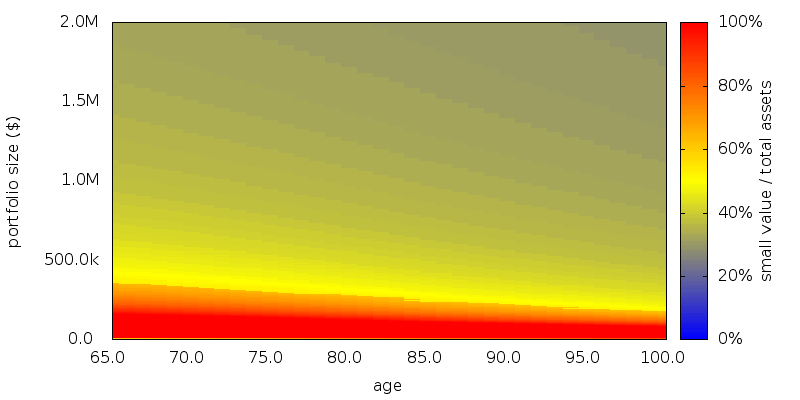
The graph below shows an abrupt lower boundary when performing asset allocation amongst 3 asset classes with variable withdrawals as detailed more fully at the end of this note. The abrupt boundary is shown in the graph by an sudden transition from yellow to orange-red:

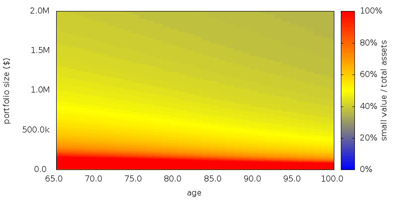
If instead of performing MVO we perform SDP on the entire multi-dimensional asset class space the abrupt lower boundary disappears:

What is more when we evaluate how well this asset allocation map performs, it does slightly better than the MVO SDP map (lifetime certainty equivalence amount $52,114 versus $52,052 for SDP with MVO). This strongly suggests the MVO efficient frontier is sub-optimal for use by SDP.

Then there is the smoking gun. If we attempt to repeat the experiment using not actual historical returns but returns generated from a distribution having the same mean, standard deviation, and correlations as the actual historical returns, but normally distributed (produced using a Cholesky decomposition), the abrupt lower boundary disappears. Additionally the two lifetime certainty equivalence amounts are now the same to within the level of noise ($51,985 versus $51,984). Thus the non-normal nature of historical returns causes SDP alone to select points off of the MVO efficient frontier.

MVO assumes returns are normally distributed, so the revelation that it is sub-optimal when returns are not normally distributed is nothing new.

The frontier

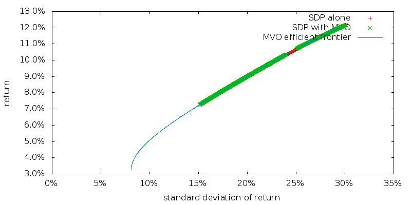
We can explore what points are used when performing asset allocation by taking all the computed asset allocation points in the region 65 <= age <= 99 and $0 <= portfolio size <= $2m. We can then compute the mean and standard deviation of the returns for each asset allocation point using the historical returns sequence. And finally plot mean versus standard deviation, or asset allocation versus standard deviation on a graph.

The mean return as a function of standard deviation of the points used by SDP alone, SDP with MVO, and the MVO efficient frontier are plotted below. The large number of points involved (56,385 map locations) causes the individual points to merge into thick lines.

And zooming in:

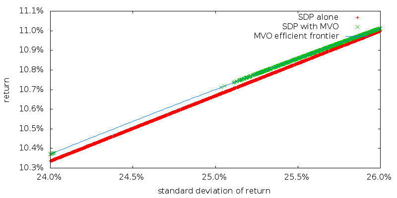
As would be expected SDP with MVO picks points on the MVO efficient frontier. While SDP alone picks points just ever so slightly below the MVO efficient frontier. The asset allocations of these two sets of points are however quite different. We will examine the readily apparent gap in points for SDP with MVO in a moment.

The asset allocations for SDP with MVO (these points lie on the MVO efficient frontier):

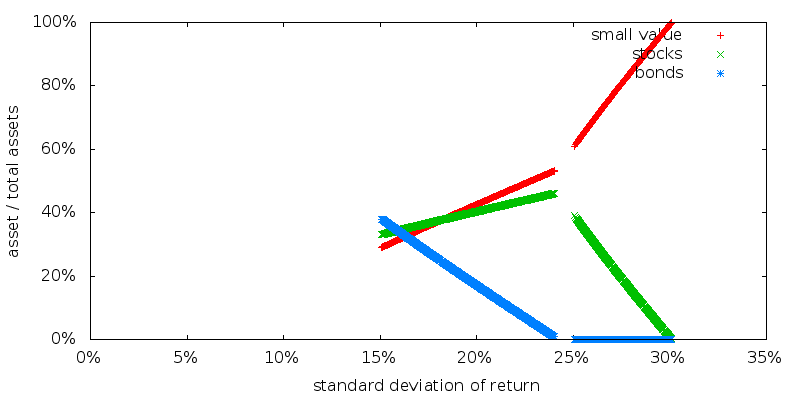
The gap that is apparent indicates that the relevant points on the MVO efficient frontier were not used by SDP, and this is consistent with the abrupt lower boundary.

The asset allocations for SDP alone (these points need not lie on any frontier):

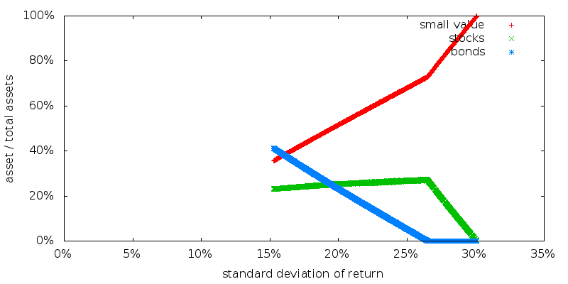
First, note the points do seem to lie on some sort of single frontier. They are not distributed at random, but form precise solid lines. And since SDP alone determines the optimal results it almost seems reasonable to describe this as an "efficient frontier". The efficient frontier for non-normal returns. Second note how different this frontier is from the MVO efficient frontier.

CARA utility

We have been using a CRRA power utility of consumption function. Switching now to SDP alone with a CARA exponential utility of consumption function gives the following asset allocations:

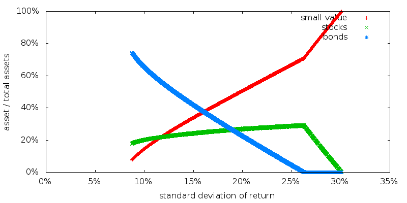
Note that the portion of the efficient frontier we use extends farther to the left, but the efficient frontier is otherwise unchanged from SDP alone with CRRA utility.

Conclusion

SO, there you have it. An apparent frontier for non-normal returns when using SDP alone that appears to be independent of the choice of consumption utility function. This frontier avoids the abrupt transitions seen by SDP with MVO, and gives better lifetime certainty equivalence performance suggesting it might be termed an efficient frontier. So far we do not know if either the frontier breaks down in other situations, or if there is a single frontier that SDP will always use. How to compute this frontier, other than through brute force SDP, is also not known.

Scenario

Scenario. A retired male/female couple, both age 65 with a $500,000 portfolio. $20,000 of guaranteed Social Security income is assumed. Longevity is as specified by the U.S. Social Security Cohort Life Tables for a person of the given initial age in 2013. No value is placed on any inheritance that is left. No additions to the portfolio are permitted, and withdrawals are made using the current asset allocation. Taxes were ignored. No transaction costs were assumed for rebalancing, sales, or purchases. All amounts are adjusted for inflation. No time discounting of the future is performed.

Asset allocation schemes: Rebalancing is performed annually. Returns data for 1927-2012 were used by SDP to generate the schemes. A zero consumption level of $0 was used, with 0% phase out with increasing income.

Withdrawal schemes: Withdrawal are performed annually at the start of the year.

Utility: CRRA power utility has an η of 3.0. CARA exponential utility has an α of 1e-4.

Asset classes and returns: U.S. stocks and 10 year Treasuries as supplied by Shiller (Irrational Exuberance, 2005 updated), and U.S. small value asset class as supplied by Fama and French, with no changes made except the small value asset class geometrically adjusted by -3.0% before expenses. Management expenses are 0.0%.

Evaluation: For each retirement number value 100,000 returns sequences were generated by selecting returns at random from the period 1927-2012. In evaluating each sequence we compute the full range of longevity possibilities.

Platform: An internal command line version of AACalc.com was used to generate the asset allocations, withdrawal strategies, and to simulate the portfolio performance.